Welcome to the Feature Column

---

Trees: A Mathematical Tool for All Seasons

Posted January 2006.

I hope to convince you that mathematical trees are no less lovely than their biological counterparts...

Joe Malkevitch
York College (CUNY)
malkevitch at york.cuny.edu

Mail to a friend

Print this article

 

 

Introduction

Trees have been the inspiration of poets and no one doubts the beauty of many wood sculptures nor the ubiquitous uses for lumber. The leaves of trees are beautiful and varied. Many find the spectacular fall colors of trees an inspiration and travel great distances to see the fall foliage. No wonder that mathematicians use the suggestive term "tree" for the special class of structures sampled below, where two rather different drawings of the same tree structure are shown.
 

I hope to convince you that mathematical trees are no less lovely than their biological counterparts.

 

Basic ideas

A powerful way to represent relationships between objects in visual form can be done using a mathematics structure called a graph. One uses dots called vertices to represent objects and line segments which join the dots, called edges, to represent some relationship between the object which the dots represent. For example, a chemist might draw the diagram below to represent a methane molecule:

 

In a graph the number of edges that meet a vertex of the graph is called the degree or valence of a vertex. The use of the term valence here reflects the fact that in forming molecules certain atoms "hook up" with a fixed number of other atoms. Hydrogen has a valence of 1 and carbon a valence of 4. In the graph of the methane molecule we see that the hydrogen atoms have valence (degree) 1, while the carbon atom has valence (degree) 4. The vertices of valence 1 in a tree are often known as leaves (singular: leaf) of a tree.


Another example would be:
 

Here the diagram shows a person's ancestors.

The two graphs we have just drawn are special because they lack cycles. A cycle in a graph is a collection of edges which make it possible to start at a vertex and move to other vertices along edges, returning to the start vertex without repeating either edges or vertices (other than the start vertex). The graph below has a variety of cycles, abda, adea, adfcba, and bdfcb. The cycles dbcfd and dfcbd are considered the same as the cycle bdfcb because the same edges are used. Can you find a list of all of the cycles in this graph?

 

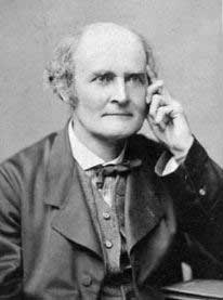
All the graphs we have drawn are also special because they have the property that given any two vertices of the graph, they can be joined by a path: a collection of edges that does not repeat any edges or vertices and that joins a vertex to a distinct vertex. For example, aedbcf is a path while adeab is not because the vertex a was repeated. A graph which has the property that any pair of vertices in the graph can be joined by a path is called connected. We will define a tree to be a connected graph which has no cycles. A pioneer in the study of the mathematical properties of trees was the British mathematician Arthur Cayley (1821-1895).

Trees have a variety of very nice properties:

a. Given two distinct vertices u and v in a tree, there is a unique path from u to v. (For technical reasons it is convenient to allow a graph with a single vertex to be a tree.)

b. If we cut (or remove) any edge of a tree, the graph is no longer connected. (Thus, trees are examples of minimally connected graphs. Connected graphs which are not trees must have edges which can be removed and still preserve the property that the graph is connected. These edges are edges that lie on cycles.)

c. If a tree has n vertices, then it has (n-1) edges. If we denote the number of edges of a graph G by |E(G)| and the number of vertices of G by |V(G)|, then |V(G)| = |E(G)| + 1. In this form this result can be thought of as a special case of Euler's (polyhedral) Formula.

d. If u and v are two distinct vertices of a tree not already joined by an edge, then adding the edge from u to v to the tree will create exactly one cycle.

It is these appealing properties of trees that give rise to the many theoretical and applied aspects of graphs which make them so ubiquitous as tools in mathematics and computer science. Trees are widely used as data structures in computer science.

Minimum cost spanning trees

One example of the power of using trees as a tool appears in a problem which often arises in operations research. Here is one applications setting. Consider the graph with weights as pictured below.
 

Each weight gives the cost of creating a communications link between the vertices at the end of the edge, so that we can send a message between the endpoints of the edges. (Edges which are omitted above have such high cost that it is prohibitive to create these links.) Our goal is to be able to send a message between any pair of vertices by selecting links in the graph above so that the weight of putting in the selected links has the smallest possible total cost. Note that we are not requiring links between every pair of vertices because if the link from A to B is inserted and the link between B and C is inserted, then one can send a message from A to C by relaying it via B. (In the interests of simplification we do not consider relay costs.) Note that if the links selected formed a cycle, one could omit the edge of the cycle with the largest weight and still be able to send messages between any pair of vertices which make up the cycle. Thus, the best answer for the network must be a tree. One is given a graph with weights on the edges, typically positive weights, though negative weights are allowed and can be thought of in applications as subsidies for the use of the edge of a graph having a negative weight. The goal is to try to find a spanning tree of the graph which has the property that the sum of the weights of the edges in the tree is a minimum. The meaning of being a spanning tree is that the tree includes all of the vertices of the original graph. (The word "spanning" in graph theory is often used for a subgraph of a graph which includes all of the vertices of the original.) Were we to select the blue edges in the diagram below as links, it would be possible to relay messages between any pair of vertices. However, can you see why this is not the cheapest way to create such a network?
 

Keep reading to see a variety of different elegant methods to find a way of choosing the links in a situation such as this which achieve minimum cost. The mathematical literature typically refers to the problem being described here as the minimal spanning tree problem or MST. This name is not ideal because one can conceive of a variety of interpretations for minimal. Here I will use the more suggestive term "minimum cost spanning tree."

History of algorithms to find minimum cost spanning trees

The history of the minimum cost spanning tree problem is rather interesting and complex. Until recently, most textbook discussions of this problem made reference to the work of two American mathematicians, then employees at Bell Laboratories, who each developed an algorithm for solving the minimum cost spanning tree problem. They are Joseph B. Kruskal who published his work in 1956,
 

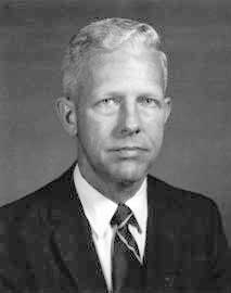
and Robert C. Prim who published his work in 1957.
 

 

In the textbook and research literature that developed concerning what Kruskal and Prim accomplished it was largely lost that others had worked on this problem previously. In particular it was mostly overlooked that in the papers of both Prim and Kruskal, reference was made to the work of the Czech mathematician Otakar Borůvka (1899-1995). Borůvka's work dated to 1926 and his algorithm for the minimum cost spanning tree problem is different from that of either Kruskal or Prim! Furthermore, Borůvka's algorithm is very elegant and deserves as much attention as that of Prim and Kruskal. His work was published in Czech (one paper with a German summary). Recent work on the history of the minimum cost spanning tree problem shows that there were a variety of independent discoveries of the algorithms and ideas involved, which is not surprising in light of the theoretical importance of greedy (making a locally best choice) algorithms and the many applied problems that can be attacked using the mathematics involved. For example, Prim's algorithm had actually been independently discovered much earlier by the Czech mathematician Vojtečh Jarník (1897-1970), who made important contributions to mathematics besides his work on trees. The complete story of the circumstances of Kruskal's and Prim's interest in the minimum cost spanning tree problem stems from problems in pricing "leased-line services" by the Bell System.

The algorithm that Kruskal discovered for finding a minimum cost spanning tree is very appealing, though it does require a proof that it always produces an optimal tree. (The analogous algorithm for the Traveling Salesman Problem does not always yield a global optimum.) Also, at the start, Kruskal's algorithm requires the sorting of the weights of all of the edges of the graph for which one seeks a minimum cost spanning tree. This requires that computer memory be used to store this information. Given computer capabilities at the time Kruskal's algorithm did not meet the needs of the Bell System's clients. It occurred to Robert Prim, Kruskal's colleague at Bell Laboratories, that it might be possible to find an alternative algorithm to Kruskal's (even though mathematically Kruskal's work was very appealing), which met the needs of the Bell System's customers. He succeeded in doing this and in noting that his method worked for graphs with ties in cost between edges and with negative weights.

All three of the algorithms due to Borůvka, Kruskal and Prim are "greedy" algorithms that is, they depend on doing something which is locally optimal (best), which "miraculously" turns out to be globally optimal.

Prim's algorithm works by picking, starting at any vertex, a cheapest edge at that vertex, contracting that edge to a single new "super-vertex" and repeating the process. Kruskal's algorithm works by adding the edges in order of cheapest weight subject to the condition that no cycle of edges is created. (One advantage of Prim's algorithm is that no special check to make sure that a cycle is not formed is required.) Borůvka's algorithm (which to work in its simplest form requires that all edges have distinct weights) works by having each vertex grab a cheapest edge. If the resulting structure is not a tree, then the components obtained are shrunk and the process repeated. The details of these algorithms are described below using a simple example.

Minimum cost spanning tree algorithms

In what follows we will use the following example (Figure 1) to illustrate the way that the various algorithms in which we are interested work. You can think of this graph as giving 6 sites that must be connected by a high transmission electrical system or a cable system of some kind. The sites that have no line segments connecting them are too expensive to connect. Note that the edges all have distinct costs (lengths), which makes the initial exposition a trifle simpler. However, the discussion below can be modified to deal with the situation in which some edges have equal weights. When there are ties for the weights of the edges, the cost associated with a minimum cost spanning tree is the same for all trees which achieve minimum cost. When the edges all have distinct weights there is a unique tree which solves the problem.

 

There are nine edges in the above graph. If we sort the weights of these edges in increasing order, we get: 4, 5, 9, 10, 11, 12, 13, 20, 24. If we try to get a cheap connecting system by adding edges in order of increasing cost, we would first insert the edges of cost 4 and 5 as shown in the diagram below:
 

The next cheapest edge would be 9 but its insertion would create a cycle. To send electricity from vertex 0 to vertex 2 does not require the link from 0 to 2 because it can instead be sent from 0 to 1 and then from 1 to 2. Hence, we need not add the link from 0 to 2. Thus, the next edges we would add would be the edges 3 to 4 and 4 to 5 because these are the cheapest at the next two decision stages. After adding these links we get the following situation:
 

 

Note that at this stage, the edges selected do not form a connected subgraph of the original edges. Thus, Kruskal's algorithm does not form a tree at every stage of the algorithm. However, by the time the algorithm terminates, the edges will form a tree. The next cheapest edge, having cost 12, would also form a cycle with previously chosen edges, so it is not added to the collection of links. However, the edge with cost 13 can be added. We now have a collection of edges which forms no cycle and which includes all the vertices of the original graph. Thus, we have found a collection of links which makes it possible to transmit electricity from any of the locations to any of the others, using relays if necessary. Since we are seeking a tree as the final collection of edges (shown in red in Figure 4), we can use the fact that all trees with the same number of vertices have the same number of edges to determine how many edges must be selected before Kruskal's algorithm, or that of Prim or Borůvka, will terminate. Specifically, we know that for a tree, the number of vertices and edges are related by the equation:
 

So that in applying Kruskal's algorithm, when we have selected a connected number of edges to put into our linking network that is one less than the number of vertices to be linked, we know that we have exactly the right number of linking edges!
 

 

Prim's algorithm is also a greedy algorithm, in the sense that it repeatedly makes a best choice in a sequence of stages. However, one difference is that Prim's algorithm always results in a tree at each stage of the procedure, producing a spanning tree at the stage where the algorithm terminates. The idea behind Prim's algorithm is to add a cheapest edge which links a new neighboring vertex (a "super-vertex") to a previously selected collection of vertices. We can choose to initiate the algorithm at any vertex of the dot/line diagram. Thus, if we start the procedure at vertex 3, we have three edges to choose from: edge 13 costing 13, edge 34 costing 10 and edge 35 costing 12. Since edge 34 is cheapest, we select this one. At this stage we have the situation shown in Figure 5:

 

We now think of shrinking the edge from 3 to 4 to a single "super-vertex." This super-vertex has neighboring vertices connected to it by edges. These are the edges 04, 13, 35, and 45 (with costs 24, 13, 12, and 11, respectively). The cheapest of these in cost is the edge 45, so we select this edge next.
 

 

At this stage we can think of vertices 3, 4, and 5 as a "super-vertex." The neighbors of this super-vertex are the edges 04, 13, and 25. Note that we do not consider the edge 35 any longer as a neighbor because it joins two vertices which are contained "within" the super-vertex. Since the edge 13, coincidentally with cost 13, is the cheapest of the neighbors of the super-vertex, we next add the edge 13 to the growing collection of links.

 

We can now continue in this way until our super-vertex consists of all of the vertices of the original graph. Here is the order in which the vertices are added to the super-vertex starting with the initial vertex 3: 4, 5, 1, 2, 0. Thus the edges added are: 34, 45, 13, 12, 10, which gives rise to exactly the same final collection of connecting edges as previously, as shown in red in Figure 4.

Although Kruskal's and Prim's algorithms are quite well known, until relatively recently the algorithm of Borůvka was less well known despite the fact that it was discovered earlier and is cited in the papers of both Kruskal and Prim. How does this algorithm of Borůvka work? It is carried out in stages, just as the those of Kruskal and Prim are. The method applies to dot/line diagrams with weights where all of the weights are distinct, as happens to be the case in our example. Under this assumption, note that the "grabbing" operation described below can not generate a collection of grabbed edges which form a cycle! Thus, the edges selected either form a tree or a collection of trees (i.e. a forest).

One stage of the algorithm consists of each vertex (or in later stages super-vertices) "grabbing" an edge which is adjacent to the vertex which is cheapest, without regard to edges grabbed by other vertices. Thus, since at vertex 0, the edges are 01, 02, and 04, the cheapest being 01 of weight 5, vertex 0 grabs edge 01. Vertex 1 has as adjacent edges 13, 10, and 12 and, thus, vertex 1 grabs the edge 12. Vertex 2, having adjacent edges 21, 20, and 25, grabs the cheapest edge 21, of weight 4. In a similar way, vertex 3 graphs the edge 34, vertex 4 grabs the edge 43, and vertex 5 grabs the edge 54. At this stage we have the current pattern of "grabbed edges":
 

 

If the blue edges in Figure 8 formed a tree, we would be finished. However, since they do not, we form a collection of super-vertices which arise from the sets of connected vertices which have currently formed with selected edges. We then carry out another "grabbing" stage of the algorithm. In our current example, there are two super-vertices (one consisting of vertices 0, 1, and 2 and the other consisting of vertices 3, 4, and 5). These super-vertices are linked with edges of weight 13, 20, and 24. If we call the super-vertices A and B respectively, A grabs the edge AB of weight 13, and B graphs the edge BA (which is, of course, the same as AB) of weight 13. This new edge, when changed to color blue, together with the blue edges in Figure 8 gives rise to the connecting edges shown in red in Figure 4. Again, we have found the minimum cost spanning tree.

Let me briefly comment on the issue of what happens for these algorithms when there are edges with the same weight in the graph for which we are trying to find a minimum cost spanning tree. The graph in Figure 9 shows an especially simple situation, but it will help clarify the situation.
 

 

In Figure 10, we have shown three copies of the graph in Figure 9, each with a minimum cost spanning tree of cost 102. This illustrates the fact that a graph which has edges with equal weights can have many minimum cost spanning trees, but that one can prove that all of the minimum cost spanning trees have the same cost. Also note that in each case the edge with maximum cost in the original graph can be part of a minimum cost spanning tree. However, in any cycle in a graph for which one seeks a minimum cost spanning tree, if the edges of this cycle have different costs, then the edge of maximum cost in this cycle can not be part of a minimum cost spanning tree.
 

I have not indicated proofs for the above algorithms. Obviously, it is important to provide such proofs. What is intriguing is that where the greedy algorithms of Kruskal and Prim are optimal for the problem of finding a minimum cost spanning tree, the analogous greedy algorithms for finding a solution to the Traveling Salesman Problem are not optimal.

The idea behind one proof of Kruskal's algorithm is to assume there is a tree T with a cost less than or equal to that of a tree K that is generated by Kruskal's procedure. Construct the list L of the edges of the tree K in the order in which Kruskal's algorithm inserted them into K. If T is not the same tree as K, find the first edge e in list L which is an edge of K but not of T. When e is added to T, because of a property of trees mentioned at the start, a unique cycle is formed. This cycle must contain at least one edge e' not in K since K, being a tree, has no cycles. Now form the tree T' which consists of adding e to T and removing e'. The cost of this new tree T' is the cost of T plus the weight on e minus the weight on e'. Since T is a cheapest tree and since Kruskal's algorithm chooses edges in order of cheapness subject to not forming a cycle, the weight on e and e' must be equal. This means that T' and T have the same cost, and, thus, K and T' agree on one more edge than K and T in terms of cost. Continuing in this way we see that we may have different trees that achieve minimum cost (these arise from different ways of breaking ties when Kruskal's algorithm is applied) but none that can be less costly than the tree that Kruskal's method produces.

One natural consideration in comparing the algorithms which have been discussed concerns the question of which of the approaches is computationally better. This turns out to be a complicated question which depends on the number of vertices and edges in the weighted graph. Questions arise concerning the computational complexity of these algorithms in terms of the data structures that are used for representing the graph and its weights, and the nature of the computer (e.g. serial or parallel) that is doing the calculations.

Although the minimum cost spanning tree algorithms were created in part due to applications involving the creation of various kinds of networks (e.g. phone, electrical, cable), many other applications have been developed. One natural extension of the mathematical model we have just been considering is to have not only a weight on the edges of the graph but also a weight on the vertices of the graph. If a vertex is part of a spanning tree where the degree (valence) of the vertex in that tree is more than one, then relays will perhaps be necessary at that vertex. In this model we seek that spanning tree of the original graph such that the sum of the weights on the edges of the spanning tree T together with the sum of the weights at the vertices of T is a minimum. Unlike the initial model where we found a variety of elegant polynomial time algorithms, this probably more realistic problem is not known to have a polynomial time algorithm. In fact, the problem is known to be NP-Complete, which suggests that a "fast" algorithm for solving this problem may not be possible.

Let us conclude with another, perhaps unexpected, extension of this circle of ideas: Minimum cost spanning trees for points in the Euclidean plane where the cost associated with a pair of points is the Euclidean distance between them. For three points forming the vertices of an equilateral triangle with side length 1, if we restrict ourselves to a spanning tree of the graph formed by the vertices and edges of the equilateral triangle, the minimum cost spanning tree will have a cost of 2. However, if we are allowed to add a fourth point P in the interior of the triangle, which when joined to the vertices of the triangle creates three equal 120 degree angles, then the three segments which join P to the vertices of the triangle, sum to a length of less than 2! The point P is called a Steiner point with respect to the original three. Problems which involve finding minimum cost spanning trees for points in the Euclidean plane when one is allowed to add Steiner point turns out to be both interesting and complex, with many theoretical and applied ramifications. Steiner trees are no less fascinating than minimum cost spanning trees.

References

Bazlamacci C. and K. Hindi, Minimum -weight spanning tree algorithms: A survey and empirical study, Computers & Operations Research, 28 (2001) 767-785.

Bern, M. and R. Graham, The shortest network problem, Scientific American, 1989, p. 66-71.

Blum, A. and R. Ravi, S. Vempala, A constant-factor approximation algorithm for the k-MST problem, Proc. 28th Symposium Theory of Computing, 1996.

Borůvka, O. jistem problemu minimalmim, Praca Moravske Prirodovedecke Spolecnosti, 3 (1926) 37-58 (in Czech)

Cayley, A., A theorem about trees, Quart. J. Math., 23 (1889) 376-378.

Chan, T., Backwards analysis of the Karger-Klein-Tarjan algorithm for minimum spanning trees, Information Processing Letters, 67 (1998) 303-304.

Chazelle, B., A minimum spanning tree algorithm with inverse-Ackermann type complexity, J. ACM, 47 (2000) 1028-1047.

Chazelle, B. and R. Rubinfeld, L. Trevisan, Approximating the minimum cost spanning tree weight in sublinear time, SIAM J. Computing, 34 (2005) 1370-1379.

Cheriton, D. and R. Tarjan, Finding minimum spanning trees, SIAM J. Computing, 5 (1976) 724-742.

Cole, R. and P. Klein, R. Tarjan, A linear-work parallel algorithm for finding minimum spanning trees, Proceedings of SPAA, 1994.

Dijkstra, E., Some theorems on spanning subtrees of a graph, Indag. Math., 22 (1960) 196-199.

Dixon, B. and M. Rauch, R. Tarjan, Verification and sensitivity analysis of minimum spanning trees in linear time, SIAM J. Computing, 21 (1992) 11-84-1192.

Du, D.-Z. and F. Hwang, A proof of the Gilbert-Pollak conjecture on the Steiner ratio, Algorithmica, 7 (1992) 121-135.

Dutta, B. and A. Kar, Cost monotonicity, consistency and minimum cost spanning tree games, Games Economic Behavior, 48 (2004) 223-248.

Fredman, M. and R. Tarjan, Fibonacci heaps and their uses in improved network optimization algorithms, J. ACM, 34 (1987) 596-615.

Fredman, M. and D. Willard, Trans-dichotomous algorithms for minimum spanning trees and shortest paths, J. Comput. Syst. Sci., 48 (1994) 424-436.

Gabow, H. and Z. Galil, T. Spencer, R. Tarjan, Efficient algorithms for finding minimum spanning trees in undirected and directed graphs, Combinatorica, 6 (1986) 109-122.

Gilbert, E. and H. Pollak, Steiner minimal trees, SIAM J. Applied Math., 16 (1968) 1-29.

Eppstein, D. and Z. Galil, G. Italiano, Dynamic graph algorithms, in Algorithms and Theory of Computation Handbook, M. Atallah, editor, CRC, Boca Raton, 1999.

Graham, R. and P. Hell, On the history of the minimum spanning tree problem, Ann. Hist. Computing, 7 (1985) 43-57.

Gusfield, D., Algorithms on Strings, Trees, and Sequences - Computer Science and Computational Biology, Cambridge U. Press, New York, 1997.

Hansen, P. and M. Zheng, Shortest shortest path trees of a network, Discrete Applied Math., 65 (1996) 275-284.

Hochbaum, D., Approximation Algorithms for NP-Hard Problems, PWS Publishing, 1997.

Hu, T., Optimum communication spanning trees, SIAM J. Computing, 3 (1974) 188-195.

Hwang, F. and D. Richards, P. Winter, The Steiner tree problem, Ann. Discrete Math. 53 (1992).

Jarník, V., O jistem problemu minimalnim (in Czech), raca Moravske Prirodovedecke Spolecnosti, 6 (1930) 57-63.

Kar, A., Axiomatization of the Shapley value on minimum cost spanning tree gamse, Games Economic Behavior, 38 (2002) 265-277.

Karger, D. and P. Klein, R. Tarjan, A randomized linear-time algorithm to find minimum spanning trees, J. ACM, 42 (1995) 321-328.

King, V., A simpler minimum spanning tree verification algorithm, Algorithmica, 18 (1997) 263-270.

Ivanov, A. and A. Tuzhilin, Minimal Networks: The Steiner Problem and its Generalizations, CRC Press, Boca Raton, 1994.

Korte, B. and J. Nesetril, Vojtech Jarník's work in combinatorial optimization, Discrete Mathematics, 235 (2001) 1-17.

Komlos, J., Linear verification for spanning trees, Combinatorica, 5 (1985) 57-65.

Korte, B. and L. Lovasz, R. Schrader, Greedoids, Springer-Verlag, Berlin, 1991.

Kou, L. and G. Markowsky, L. Berman, A fast algorithm for Steiner trees, Acta. Inform., 15 (1981) 141-145.

Kruskal, J., On the shortest spanning subtree of a graph and the traveling salesman problem, Proc. Amer. Math. Soc., 7 (1956) 48-50.

Kruskal, J., A reminiscence about shortest spanning trees, Archivum Mathematicum (BRNO), 33 (1997) 13-14.

Lavallée, I., Un algorithm parallèle efficace pur construire un arbre de poids minimal dans un graphe, RAIRO Rech. Oper., 19 (1985) 57-69.

Leeuwen, J. van, Graph Algorithms, in Handbook of Theoretical Computer Science, J. van Leeuwen, (editor), Volume A, Algorithms and Complexity, MIT Press, Cambridge, 1994.

Levcopoupoulos, C. and A. Lingas, There are planar graphs almost as good as the complete graphs and as cheap as minimum spanning trees, Algorithmica, 8 (1992) 251-256.

Nesetril, J., A few remarks on the history of the MST problem, Archivum Mathematicum (BRNO), 33 (1997) 15-22.

Nesetril, J. and E. Milová, H. Nesetrilova, Otakar borůvka on minimum spanning tree problem: Translation of both the 1926 papers, comments, history, Discrete Mathematics 233 (2001) 3-36.

Pettie, S. and V. Ramachandran, An optimal minimum spanning tree algorithm, J. ACM, 49 (2002) 16-34.

Pollak, H., Private communication, 2005.

Prim, R., Shortest connection networks and some generalizations, Bell. System Tech. J., 36 (1957) 1389-1401.

Prim, R. Personal communication, 2005.

Promel, H. and A. Steger, The Steiner Tree Problem, Vieweg, Braunschweig/Wiesbaden, 2002.

Ravi, R. and R. Sundaram, M. Marathe, D. Rosenkrantz, S. Ravi, Spanning trees short or small, SIAM J. Discrete Math., 9 (1996) 178-200.

Rosen, K., (editor), Handbook of Discrete and Combinatorial Mathematics, Chapter 9 (Trees), Chapter 10 (Networks and Flows), CRC, Boca Raton, 2000.

West, D. Introduction to Graph Theory, Second Edition, Prentice-Hall, Upper Saddle River, 2001.

Wu, B.-Y. and K.-M. Chao, Spanning Trees and Optimization Problems, Chapman & Hall/CRC, Boca Raton, 2004.

Xu, Y. and Volman, D. Xu, Clustering gene expression data using graph theoretic approach: An application of minimum spanning trees, Bioinformatics, 18 (2002) 536-545.

Yao, A. An O(|E| log log |V|) algorithm for finding minimum spanning trees, Info. Processing Lett., 4 (1975) 21-23.

Joe Malkevitch
York College (CUNY)
malkevitch at york.cuny.edu

---

NOTE: Those who can access JSTOR can find some of the papers mentioned above there. For those with access, the American Mathematical Society's MathSciNet can be used to get additional bibliographic information and reviews of some these materials. Some of the items above can be accessed via the ACM Portal, which also provides bibliographic services.