How to Make a 3D Print
Mathematically speaking, the 3D print is constructed from a 1-dimensional path. This article will describe how to find that path...
Introduction
We frequently hear that we are in the midst of a 3D printing revolution. Indeed, a recent story on the PBS Newshour compellingly demonstrates how 3D printing is being used in a wide range of areas from medicine to the arts.
Though some of the claims may sound overblown, my experience as a mentor to a team of high school students preparing for a robotics competition shows how simple it is to 3D print custom parts and prototype ideas quickly and efficiently.
After using the printer for a while, I began to wonder how the process works. Each print is created layer by layer from a spool of plastic filament that is slightly melted and extruded from a nozzle moving along a planar path. Mathematically speaking, the 3D print is constructed from a 1-dimensional path. This article will describe how to find that path.
To be more specific, most 3D prints begin as a file written in the STL (stereolithography) format. Most STL files are created by 3D design software though the format is simple enough for you to write them yourself. For instance, here is a piece of an STL file:
facet normal -6.123234e-17 0.000000e+00 1.000000e+00

	outer loop

	vertex -6.514841e+00 1.043095e+02 9.525001e+00

	vertex -9.595548e+00 1.042182e+02 9.525001e+00

	vertex -6.558662e+00 1.041282e+02 9.525001e+00

	endloop

	endfacet

	facet normal -6.123234e-17 0.000000e+00 1.000000e+00

	outer loop

	vertex -6.558662e+00 1.041282e+02 9.525001e+00

	vertex -9.595548e+00 1.042182e+02 9.525001e+00

	vertex -9.541054e+00 1.040397e+02 9.525001e+00

	endloop

	endfacet
In this format, the boundary of the solid is described as a list of triangles, each of which is specified by stating its three vertices and a normal vector. This file is converted into a set of instructions in G-code, a language widely used in numerical control machines, and these instructions are sent to the printer. Here is a bit of the G-code created from the STL file.
G1 F3300.0

	M101

	G1 X55.8 Y0.0 Z1.47 F1111.111 E1112.261

	G1 X58.74 Y1.8 Z1.47 F1111.111 E1112.515

	G1 X-26.47 Y1.8 Z1.47 F1111.111 E1118.807

	G1 X-26.47 Y3.6 Z1.47 F1111.111 E1118.94
The M101 command turns on the extruder while the G1 command tells the extruder to move to a specific location and the G1 F command sets the rate at which plastic is fed into the extruder.
This article will outline how the STL file is converted into G-code instructions by the RepRap Project, an open source 3D printing community project. RepRap claims to be "humanity's first general-purpose self-replicating manufacturing machine." This claim may be a bit strong, however: the printer can print many, but not all, of its own parts, and it can't assemble them. Nevertheless, the source code is freely available and easy to read, which is why it's fun to follow along.
The mechanics of 3D printing
Before we begin our description of the STL to G-code conversion process, let's look at the physical machine we will be controlling. The pictures that follow are of a MakerBot Replicator 2.
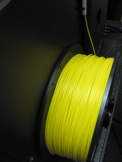 |
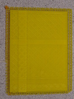
The printing material is a colored plastic filament whose diameter is 1.82mm. Of course, other 3D printers can print in a variety of media; InnoCentive is currently offering a $7000 prize to a group or individual that can design a way to use cotton fiber in a 3D printing process. |
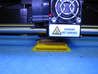 |
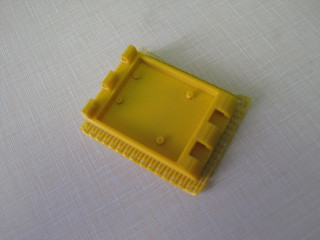
The filament is fed into the printer's write head, and melted plastic is extruded from its nozzle. |
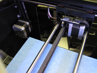 |
Three stepper motors control the location of the extruder nozzle. Two motors control the motion of the nozzle in two perpendicular horizontal directions ($x$ and $y$), while a third motor controls the vertical position ($z$) of the platter on which the filament is deposited. |
 |
A fourth stepper motor controls the rate at which plastic is fed into the extruder, but this will not concern us here. Stepper motors may only move to a discrete set of locations, which determines the resolution of the 3D print. For instance, the Replicator 2 has a layer resolution of 0.1 mm.
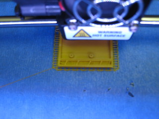
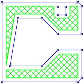
The print is constructed one layer at a time. That is, all the plastic is placed for the lowest $z$ value, the platter moves down one level, and the next layer is printed. When printing a layer, the printer first moves around a set of polygonal curves defining the boundary of that layer.
|
 |
Then the interior of the polygonal curves are filled with a cross hatching pattern to create the solid. A parameter in the printing software allow the user to set how much of the interior is filled. |
 |
Here's the final print. |
With this outline under our belt, let's start digging into the algorithm that creates G-code.
Comments?
Slicing the solid into polygons
Remember that our STL file contains a list of triangles that form the boundary of the solid we are printing. It is important to note that there could be a huge number of triangles since our design software will approximate a curved surface with many triangular patches.
|
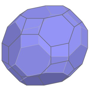
Suppose we would like to print this truncated cuboctahedron. |
 |
|
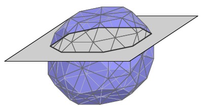
The solid is represented in the STL file as a set of triangular faces. The vertical stepper motor determines the $z$ coordinates of the layers to be printed so we will slice the solid by the corresponding planes. Let's focus on the construction of a single layer.
|
|
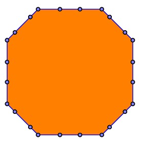
Ignoring a few subtleties, each triangle is sliced by this plane to obtain a collection of line segments. Ideally, this will produce a set of polygonal curves describing a planar region to be filled. |
 |
|
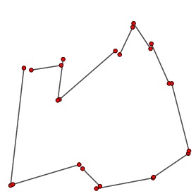
In practice, however, numerical error occurs when computing the endpoints of the line segments so they do not fit together perfectly to form a curve. In fact, it may be unclear how the line segments connect with one another to form the polygonal boundary curves. |
 |
|
Our task is to assemble all the line segments into sets of polygonal paths. It may seem that the best strategy would be to identify each vertex with its nearest vertex. However, if vertex $A$ has $B$ as its nearest neighbor, it may not be the case that $A$ is $B$'s nearest neighbor. In addition, searching for the nearest neighbor is computationally intensive.
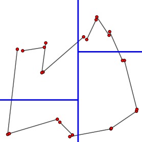
For this reason, we will employ a quadtree to determine which vertices should be identified. We first divide the region horizontally so that half the points are on the left and half are on the right. Next we divide each of the sides vertically so that an equal number of points are found above and below. This operation is made easier by first sorting the points horizontally and vertically.
|
 |
|
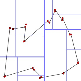
This process creates four rectangular regions, each of which we study independently. If a rectangular region has exactly two vertices, then these should be identified. If not, we continue the subdivision process.
Eventually, each rectangular region has exactly two vertices.
|
 |
|
Identifying these pairs of vertices leads to the polygonal curve as shown. |
 |
|
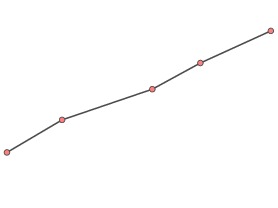
Since the segments in the polygonal curve are computed from the intersection of the slicing plane with a large number of triangles, it is likely that we have divided a straight line segment into many small pieces that don't perfectly line up. |
 |
|
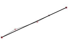
These may be detected and replaced by a single line segment. |
 |
Now that we have determined the set of polygonal curves that arise as the intersection of the current slicing plane with the solid, we arrive at an interesting problem. Suppose one layer of our solid looks like this.
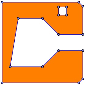
It may seem that we could simply tell the extruder nozzle to trace out these polygonal curves and then fill in the interior. However, the thickness of the filament would cause the plastic to spill over the edge of the filled region so we would not be accurately rendering the slice. Instead, we need to move the path of the nozzle into the region by half the width of the filament.

As the figure shows, this can be a tricky business. Edges of the polygonal boundary may disappear, others may be broken into smaller pieces, and the topological characteristics of the region may change. Solving this problem requires some work and some interesting ideas. We will begin by describing the filled region using Constructive Solid Geometry.
Comments?
The CSG representation of a polygon
Constructive Solid Geometry, or CSG, gives us a convenient way to represent a set of points and work with it inside a computer program. In essence, CSG considers sets as being constructed from simpler sets used as building blocks and put together with a few simple rules. In our application, the building blocks are half-planes, and the simple rules for putting them together are the familiar set-theoretic operations of complement, intersection, and union.
An oriented line defines a preferred half-plane $H$ to the left of the line when moving in the direction implied by the orientation.
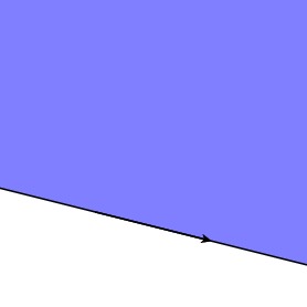
It will often be useful for us to think of $H$ as defining a boolean function on the plane: $H(p) = \hbox{True}$ if and only if $p \in H$.
The operations of intersection, union, and complement produce these results.
 |
$\left(H_1\cap H_2\right)(p) = H_1(p)\thinspace\mbox{and}\thinspace H_2(p)$ |
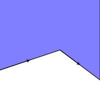 |
$\left(H_1\cup H_2\right)(p) = H_1(p)\thinspace\mbox{or}\thinspace H_2(p)$ |
 |
$\overline{H}(p) = \mbox{not}\thinspace H(p)$ |
Notice that the difference of two sets may be expressed in terms of these operations: $A \setminus B = A \cap \overline{B}$.
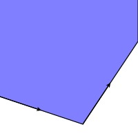
Observe that convex polygonal regions have a particularly simple expression. If we orient the edges of a convex polygon $P$ so that we travese the polygon in the counter-clockwise direction, then the polygon is given by the intersection of the half-planes defined by the edges.
|
$P=H_1\cap H_2\cap \ldots \cap H_n$ |
 |
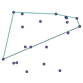
In fact, it is straightforward to describe any polygonal region in terms of convex polygonal regions. To this end, remember that the convex hull of a set of points is the smallest convex set containing that set of points. For instance, is we start with this set of points:
we find the convex hull:
As we'll see momentarily, there is a straightforward algorithm for finding the convex hull of a set of points. Now there are many possible CSG representations, and several algorithms for finding one. Since convex sets have simple CSG representations, however, we choose the following method. Suppose we would like to find a CSG representation of this region:
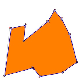
We first consider the outer polygon $P$ and find its convex hull $A$.

The fact that the original polygon $P$ is not convex is detected by traversing the convex hull and noting that we skip some of the points of $P$, which themselves form a new polygonal region.
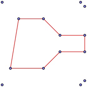
The original polygonal region $P$ is the difference in its convex hull $A$ and this new polygonal region, whose convex hull we call $B$.
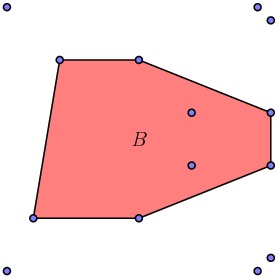
Notice again that the new polygonal region is the difference in its convex hull $B$ and the regions $C_1$ and $C_2$.
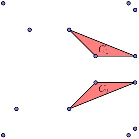
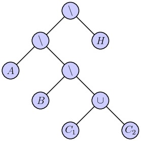
Since $C_1$ and $C_2$ are themselves convex, we arrive at a CSG representation of $P$ in terms of convex sets:
\[ P = A \setminus (B \setminus (C_1 \cup C_2)).\]
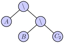
It is convenient to express this represenation as a binary tree:
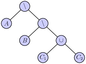
In this representation, each of the leaves of the tree are convex sets, which are described by the intersection of the half-planes defined by the edges. We therefore replace the leaves of this tree with binary trees representing the intersection of these half-planes. The result is a new binary tree whose leaves are half-planes.
This binary tree representation can be naturally constructed in our code. Furthermore, we may view this expression as a boolean-valued function on points in the plane, as we mentioned earlier. For instance, if $p$ is a point in the plane, we may now determine whether $p$ is inside $P$. Beginning with the root, we evaluate the two binary sub-trees and join them with the appropriate logical operation.
Among other things, this makes it easy to determine, by evaluating $P$'s boolean-valued function on other polygonal curves found in this layer, that there is a hole $H$ that needs to be removed.

This leads to the full tree
Comments?
The QuickHull Algorithm
We now have a way to obtain a CSG represention of a layer's filled region in terms of convex sets. All that remains is an algorithm to determine the convex hull of a set of points. The algorithm used by RepRap is called QuickHull.
|
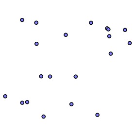
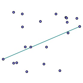
We begin with a set of points. |
|
|
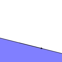
Find the points with the smallest and largest $x$ coordinates and consider the line between them. This separates the points into two smaller sets, the points below the line and those above. We will look at each set in turn. |
 |
|
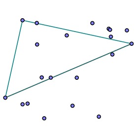
Considering the points above the line, find the point farthest from the line and use it to define two new line segments. Notice that the points inside the triangle will be inside the convex hull so they no longer need to be considered. |
 |
|
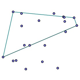
For each of the two lines we just added, consider the points above the line and find the one farthest from the line. If there is no such point, then that line segment is part of the convex hull. Otherwise, replace the line segment with two new line segments and continue. |
 |
|
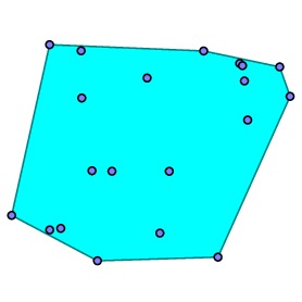
Repeat until there are no points above the line segments we have added. |
 |
|
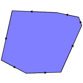
Finally, apply this process to the points below the original line to obtain the convex hull. |
|
Comments?
The boolean grid
Using our CSG representation of the filled region, we are now in position to determine the path taken by the extruder nozzle. We need one more ingredient, which we'll call a boolean grid.
Since the nozzle of our printer is positioned with stepper motors, there are only a discrete number of positions that it can visit. We will use this fact by placing a grid of points, representing these positions or pixels, on the plane.
Considering the CSG representation of our filled region as a boolean-valued function $F$ on the plane, we may determine which of the pixels are inside our region; namely, $p$ is inside the region if $F(p)$ is True.
Of course, we could determine these pixels by checking the value of the CSG expression at each pixel. However, a more efficient algorithm uses another quadtree and this simple observation: Given a rectangle $R$ and a half-plane $H$, all the points in $R$ are in $H$ if and only if the four vertices of $R$ are.
Remember the shape of our CSG tree and recall that each of the nodes $A$, $B$, $C_1$, $C_2$, and $H$ are themselves binary sub-trees representing the intersection of the half-planes defining the convex sets.
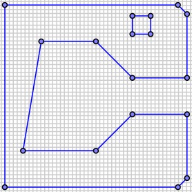
We begin by dividing our region into four rectangles and studying each in its turn.
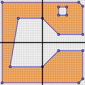
In each of the four rectangles, we may "prune" the CSG tree by evaluating each of the four vertices of the rectangle on the leaves of the CSG tree. Consider, for instance, the lower left rectangle and the lower edge of the hole $H$. Evaluating each of the four vertices of this rectangle by the half-plane defined by the lower edge of the hole $H$ gives False. In other words, there is no point in the lower left rectangle that intersects $H$. In fact, the same argument shows that no point in this rectangle intersects $C_1$. This means that, when looking in the lower left rectangle, we need only consider the smaller tree:
Even the sub-trees defined by $A$, $B$, and $C$ may be pruned since the four vertices of the rectangle evaluate to True for many of the half-planes defined by the edges of these convex sets.
We now descend this into rectangle by subdividing it into four rectangles, and consider the upper right rectangle that is created.
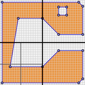
Remember that we only need to evaluate this rectangle against some of the half-planes in $A$, $B$, and $C_2$. When we do this, we see that the rectangle is contained in $B\setminus C_2$, which means that it is not inside our polygonal region. We may therefore set all the pixels inside to False.
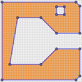
As indicated by this example, pruning the CSG tree as we move down the quadtree allows us to efficiently evaluate the boolean grid. We have now determined that the orange pixels are the ones inside the filled region.
Comments?
Shaving the boolean grid to find the nozzle path
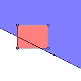
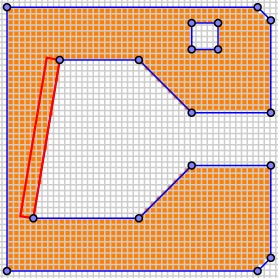
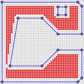
Now that we have determined the pixels inside the fill region, we may determine which pixels need to be shaved off to produce the path we want the nozzle to follow. We will denote half the width of the nozzle by $r$ so we would like to move each of the edges into the region by a distance $r$.
For each edge of our region, we create a rectangle of width $r$ and set all the pixels inside that rectangle to False. Shown below is the rectangle for one of the edges.
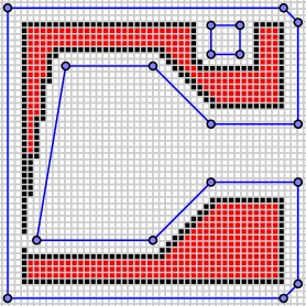
In fact, we may find the pixels inside the rectangle, as before, using a quadtree that begins with the bounding box of the rectangle.
Around each vertex, we also shave off a circle of radius $r$. This results in a new boolean grid.
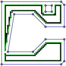
From this point, we identify the nozzle path by finding the pixels on the boundary that are not surrounded by pixels in the region.
The nozzle path is determined by walking around this boundary. Rather than ask the nozzle to move from boundary pixel to adjacent boundary pixel, an algorithm is applied to determine when a set of adjacent pixels are sufficiently close to lying on a straight line. This results in the final nozzle path.
Comments?
Cross-hatching
At last, we have found the nozzle path that outlines the boundary. Since we are creating a solid, we also need to determine how to fill it in. In many 3D printers, we are able to specify how much of the interior, a percentage perhaps, we want filled. The printer uses this percentage to create a cross-hatch pattern.
Given our CSG representation of the region, this is fairly simple. Begin by considering all the possible grid lines.
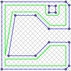
For each grid line, we determine the intersection points with the boundary path and order the points along the line. For each segment joining two adjacent intersection points, we then use the CSG representation of the region to determine whether the midpoint of the segment is in the region and, hence, whether the segment should be traced by the printer.
Comments?
Summary
In describing this process, I have made a number of simplifications, but this outline gives the essential ingredients. There are also, at several steps in the process, different choices that one could make.
The CSG representation of the fill region is not unique, and, in fact, there are representations that may be obtained and used more efficiently. I have described this representation since it is the one used by RepRap and it is relatively simple to explain. An alternative representation, in which each edge of the polygon is used exactly once, is given in the references (Dobkin, et al).
The problem of finding the nozzle path from the polygonal curves may also be solved in other ways. The method using a boolean grid exploits the fact that our 3D printer has a specific resolution. Another solution, which has a more geometric flavor, is also given in the references.
Comments?
References
-
RepRap Home Page.
-
RepRap Wiki. This site contains an overview of the process described in this article.
-
The RepRap Project software repository. You can read the source code here.
-
David Dobkin, Leonidas Guibas, John Hershberger, Jack Snoeyink. An efficient algorithm for finding the CSG representation of a simple polygon. Computer Graphics (Proceedings of SIGGRAPH 88) 22(4): 31-40, August 1988.
This paper presents an alternative method for finding the CSG representation of a simple polygon. The resulting representation uses only edges of the polygon and each edge is used only once.
-
C. Bradford Barber, David P. Dobkin, Hannu Huhdanpaa. The quickhull algorithm for convex hulls. ACM Transactions on Mathematical Software 22 (4): 469–483. 1995. Available at this site.
-
Avraham Melkman. On-line construction of the convex hull of a simple polyline. Information Processing Letters. 25 (1): 11-12. 1995. Available at this site.
Melkman's algorithm for finding the convex hull of a simple polygon is often considered to be the best such algorithm.
-
Hyun-Chul Kim, Sung-Gun Lee, Min-Yang Yang. A new offset algorithm for closed 2D lines with islands. International Journal of Advanced Manufacturing Technology. (2006) 29 : 1169-1177. Available at this site.

 David Austin