Pretty as a Picture (Part I)
In honor of Mathematics and Statistics Awareness Month I will try to show how pictures of equations of algebraic expressions inspired and continue to inspire...
 Joseph Malkevitch
York College (CUNY)
Email Joseph Malkevitch
Introduction
While not all pictures may be worth a thousand words, many geometers and other mathematicians find pictures inspire mathematical thoughts. And perhaps some in the general public might enjoy seeing images that inspire mathematics rather than complex equations that are often used to carry out mathematical thought and practices. In honor of Mathematics and Statistics Awareness Month I will try to show how pictures of equations of algebraic expressions inspired and continue to inspire, and hopefully make these algebraic equations less mysterious.
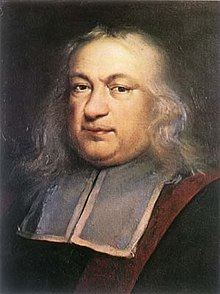
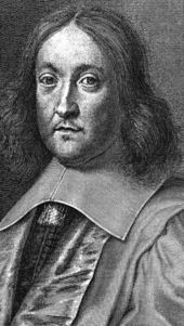
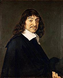
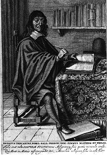
Remarkably, the dramatic developments in geometry done in ancient Greece and reflected in the Elements of Euclid were unified and reinforced with the development of analytical geometry by Fermat (1607-1665) and Descartes (1596-1650).
Figure 1 (Two portraits of Pierre de Fermat. Courtesy of Wikipedia.)
Figure 2 (Two images of Descartes. Courtesy of Wikipedia.)
This wedding between geometry and algebra via the subject called analytical geometry has been to the great benefit of both of these mathematical domains, not to mention all other mathematical domains. Thus, someone might draw a picture of a circle or an ellipse but now one also has a way of using an "algebraic formula/equation" to represent the picture. Mathematicians can write down equations and look at what they represent as well as seek out equations for "pretty" curves in the hope that the equations will show some pattern that will lead to additional mathematical insights. Some of the curves we will explore have associations with famous mathematicians and you can find examples of such associations in this bibliography of curves. Sometimes these curves are defined by "verbal" descriptions that allow mathematicians to derive equations for the graphs of the algebraic expressions which represent these graphs. For example, an ellipse results from looking for those points in the Euclidean plane, the sum of whose distances from two fixed points (called the foci of the ellipse) is a constant. However, ellipses also arise from cutting right circular cones with a plane in a particular way.
If you sent someone or received a Valentine's Day Card on Feb. 14 you might enjoy this image

Figure 3 (Image for Valentine's Day. Courtesy of Wolfram/Alpha.)
which arises from plotting those pairs $(x,y)$ that satisfy this equation:
Plotting Points
Those familiar with Cartesian coordinates and lines can move to the next segment, Conic sections. Let me briefly review the framework for converting algebraic expressions to pretty pictures. One can admire the pictures below, however, without these "details." Pretty pictures of graphs of equations rely on the notation that one can represent a point in two dimensional space (a flat piece of paper or a computer screen) by using two numbers to represent a point. In d-dimensional space one would need d numbers to represent a point, but beyond two-dimensions things are much more complicated because one can't represent what one draws with relative ease on a flat piece of paper. In modern times, one begins with two lines which meet at right angles called coordinate axes. Traditionally (Figure 4 ) the vertical line is called the y-axis and the horizontal line is called the x-axis.
Each axis can be thought of as in two halves. The y-axis has a half above the point where the lines intersect (called the origin); one lays out along that part a number scale with positive whole number values (equally spaced from each other) and along the other half, negative whole numbers (equally spaced). The positive values are in the up direction on the line and the negative numbers in the down direction from the origin. For the x-axis one lays out positive numbers to the right and negative numbers to the left of the origin. Each point is represented by an ordered pair of numbers $(x,y)$. The pair $(x,y)$ are called the coordinates of the point. Thus, (2, -3) represents a point with x-coordinate 2 and y-coordinate -3. The numbers in a pair can be any real numbers but in the diagram below the coordinates are usually integers, either positive or negative whole numbers. The point where the two axes meet is assigned the pair (0, 0). If one wants to locate where the point (2, -3) should be placed, one imagines oneself at (0, 0) and treats the pair (2, -3) as "motion directions." Since the x value of the pair is positive 2, walk two units to the right (now one is at the point (2, 0)) and then one walks down (since the second coordinate is negative) 3 units. Other examples of points can be similarly plotted as in Figure 4.
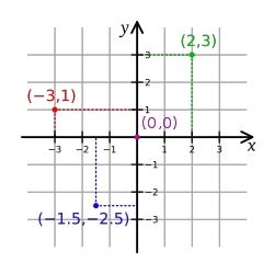
Figure 4 (Plotting points using a pair of orthogonal (meeting at right angles) axes. Diagram courtesy of Wikipedia.)
If one has an equation involving x and y, one can put a point in a diagram such as that in Figure 4 at each point whose coordinates $(x,y)$ satisfy the equation. Thus, the equation $x = 0$ is satisfied by the points (0, -11), (0, -2), (0, 0), (0, 7), as well as infinitely many other ordered pairs whose first coordinate is zero. Thus, $x = 0$ is the equation of the points that lie on the vertical line we are calling the y-axis. The x-axis consists of all points which satisfy the equation $y = 0$. More generally the horizontal lines have equations like $y = 2$ or $y = -6$ while vertical lines have equations like $x = -3$ or $x = 3/4$.
The simplest equations in x and y are those that have only the first power of x and y appearing, rather than terms like $x^2$ or $y^2$. The most general form of such equations is $ax + by + c = 0$, where the letters a, b, and c, are "fixed" constants but can take on values independent of each other. We have already seen the special cases of this equation when a or b (but not both) is zero, lead to lines that coincide with or are parallel to the coordinate axes lines. However, it is not hard to see that in general $ax +by + c = 0$ (a and b not both zero) are straight lines.
When $c = 0$ these lines go through the point (0,0) since for any choice of a and b we can compute using the equation that $a(0) + b(0) + 0$ evaluates to 0. So (0, 0) is on the family of lines where $c = 0$. In what follows we will always think of lines (e.g. $ax + by + c = 0$) or graphs of other equations that we might write down as being drawn with respect to a set of coordinate axes such as the ones shown in Figure 4. When drawing a line that does not pass through (0, 0) it is helpful to find the "intercepts" of the line, when the line intersects the x-axis (a point of the form $(u, 0)$) and the y-axis (a point of the form $(0,v)$). Remember that two points determine a unique line.
Lines are fundamental to many elementary and advanced concepts in mathematics. The term line is usually reserved for a shape that when graphed goes off to infinity in two directions, so when we draw lines on a piece of paper we can only show a part of a line. Note that two different equations may have the same graph. Thus, $x + y - 4 = 0$ and $2x + 2y - 8 = 0$ have the same graph. The issue boils down to a common concern in mathematics: when are two things "the same" and when are they "different"? The values of $(x,y)$ that satisfy an equation do not change if we multiply that equation by a non-zero constant. Also, the set of points (pairs $(x,y)$) that satisfy the equation $x + y - 5 = 0$ is the same set of points (pairs $(x,y)$) that satisfy the equation $x + y = 5$ or the equation $y + x = 5$ or $y + x - 5 = 0$. The reason we learn to manipulate equations to get equivalent equations algebraically, something many people find "painful," is that it allows us, among other things, to see what equations will have the same graph. Thus, it is helpful when plotting the graph of the equation:
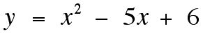
(*)
that the graph of this equation is the same as the graph of $y = (x-3)(x-2)$. We have used the tool of "factoring" the expression on the right hand side of (*). From the factored form it is easier to see that the graph of (*) passes through the point (3, 0) and the point (2, 0). When x is zero one sees that y must be 6, so the graph also passes through (0, 6). It turns out that this equation represents a particular example of a parabola. Once one sees the magic of analytical geometry lots of what is done in algebra for some people makes a lot more sense and certainly is very useful for connecting algebra to geometry via analytical geometry. Many very interesting curves can be gotten with equations that use trigonometric functions, logarithmic, or exponential functions, in addition to the more familiar algebraic functions. Here I will only consider examples involving polynomial equations, similar to the equation in (*).
Technical note:
The coordinate system used above is often called Cartesian or a rectangular coordinate system. As a matter of historical interest, Descartes did not actually use a system where there were four quadrants, but used only what today would be called the first quadrant, where the values of x and y are both positive. One could also use what are called polar coordinates to write down equations and get interesting pictures, too. Polar coordinates rely on ideas from trigonometry. Another type of coordinate system would be to use homogeneous coordinates for points and work in what is sometimes called the real projective plane. In this geometry a point would be represented by a triple $(x, y, z)$ with not all three of the coordinates zero, and where two triples of coordinates represent the same point when one is a non-zero multiple of the other. Thus, in this coordinate system (1, 2, 1) and (2, 4, 2) would be the same point. One of many advantages of this approach is that the asymmetry between (1, 2) and (2, 4) being different points while $x + 2y = 0$ and $2x + 4y = 0$ are the same lines (Euclidean case) does not occur. In this coordinate system a line has the "homogeneous equation" $ax +by +cz =0$ rather than the equation $ax + by + c = 0$. For a very brief primer of these ideas look here.
It should be intuitively clear that if we graph two lines that are not sitting on top of each other, the two lines have the same shape. This means that one can either shift (translate) one line onto the other (in which case the lines are called parallel lines) or one can locate the point where the two lines intersect and rotate one of the lines about that point until the line coincides with the other line. Given a single point, like the origin, there are infinitely many lines that pass through this point (e.g. $x - y = 0; x - 3y = 0$). However if one picks any two different points, there is only a single line that passes through them. There are different ways to obtain the equation of the line that passes through two points, say $(x_0, y_0)$ and $(x_1, y_1)$. However, it is especially helpful to see this in the equation:
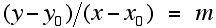
The constant m is known as the slope of the line. Vertical lines, lines with equations of the form $x =k$, have undefined slope. Part of the reason for interest in the concept of slope is that when Newton and Leibniz developed the ideas that became what today is called Calculus, they used the notions of slope of a line and the concept of tangent line to a curve as part of how to conceptualize about derivatives. The derivative helps one understand the important concept of rate of change. Rates of change come up in physics, chemistry, biology and economics but though Calculus has many applications it has internal questions of interest in its own right. In addition, to understand the "shape" of lines, analytical geometry is also concerned with understanding the "essence" of the properties that make a circle a "circle" or an ellipse a shape different from a "hyperbola."
Conic sections
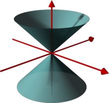
An interesting type of graph which came to be studied in ancient times is known as the hyperbola. Apollonius wrote a book about the conics over 2000 years ago! Hyperbolas are a special kind of interesting class of curves that arise as "conic sections." Figure 5 shows the two napes of a "right circular" cone, where the vertical "axis" of the cone is perpendicular to the "horizontal" plane determined by the intersection of the lines formed by the two rays in the middle of the diagram.
Figure 5 (Two napes of a right circular cone. Courtesy of Wikipedia.)
When this cone is cut by various planes one gets points that lie in the intersection of the cone and the plane. When the intersection of the plane and the cone is 2-dimensional one can get a circle, an ellipse, a parabola or the two pieces of a single hyperbola (one on the upper part of the cone and one on the lower part). I will postpone until later that one can cut a cone in a very special way to get a single point or a single line, which are often called degenerate conic sections. I will say more about them below.
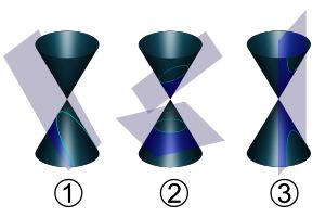
Figure 6 (Conic sections; in 1, a parabola; in 2, a circle and an ellipse, and in 3. a hyperbola. Diagrams courtesy of Wikipedia.)
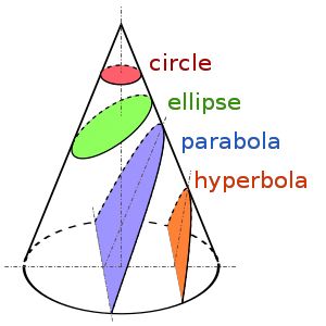
Figure 7 helps clarify how some of the different kinds of conic sections arise from plane sections of one nape of a cone when the plane is at different angles to the axes and generating lines of the cone.
Figure 7 (Schematic of conic sections. Courtesy of Wikipedia.)
All Euclidean distance circles (round) of the same radius are congruent, that is, if they are moved without "distortion," any circle of radius r can be superimposed on any other circle of radius r. However, it may seem mysterious that the same circle has different equations depending on where the coordinate system is placed with regard to the circle.
A circle referred to a pair of orthogonal (meet at right angles) axes at the point (0,0) has the equation below. The center of the circle is at (0, 0) the origin.
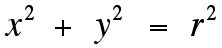
(1)
But the same (congruent) circle, with center at the point (-5, 2) has the equation
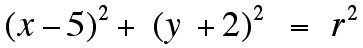
(2)
Given such equations one can look for points that satisfy the equation and thus lie on the graph of the curve that the equation defines. A complication is that there are numbers that satisfy equations that are not real numbers and there are equations which have no real number solutions. Thus,
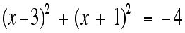
(3)
has a very similar appearance to that of the circle of radius r in (2). However, for real numbers when one multiplies such a number by itself (e.g. 3 or -7) the result is always positive ($3 \times 3 = 9; (-7)(-7) = 49$). Furthermore, adding positive numbers can only yield a positive number. So there are no real numbers x and y which satisfy (3). There are "complex numbers" (numbers of the form u + vi where i is the square root of -1) which satisfy (3) but here we will not take on the interesting question of "graphing" the solutions of equations which involve complex numbers. By the way, it is worth noting that when the right-hand side of (2) is zero, the only solution of the equation shown is (5, -2) which can be thought of as a degenerate circle with radius 0.
One can now try to study, by way of example, a particular curve, say the hyperbola. Just as circles can differ because they have different radii, hyperbolas can be "congruent" to each other (if one moves one curve without "distorting" it, one can superimpose it on another curve in a different location) but they can also differ in shape. In Figure 8 the different colored curves are not congruent, though they all "look" like hyperbolas. Different shaped curves in the same family will have different equations. The equations $y = 4/x$ and $y = 20/x$ are not congruent but are each hyperbolas, and the change of constant results in the change of one hyperbola of the family to another. But those of you who have studied a bit of analytical geometry (or Calculus) may not recognize equations like $y = A/x$ as graphs of hyperbolas.
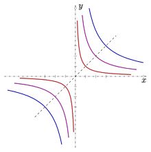
Figure 8 (Three hyperbolas $y = A / x$ where each separate color coded graph never touches the two axes though they get closer and closer to the lines $y = 0$ and $x =0$, a phenomenon described by saying each hyperbola is asymptotic to the coordinate axes. Color code: red: A=1, magenta: A=4; blue: A=9. Image courtesy of Wikipedia.)
You perhaps might recognize the equation
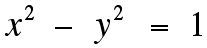
(4)
as being that of a hyperbola. To get a more familiar equation for the hyperbolas in the family $y = A/x$ one can transform the equations by conducting a rotation of the axes shown Figure 8. If one refers the curves to the 45-degree angle line shown there, and a line is drawn through (0, 0) perpendicular to that line, one will get a more familiar equation for the hyperbolas involved:
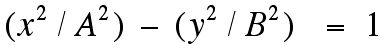
(5)
We can rewrite the equation $y = A/x$ as $xy = A$. For each point on the hyperbola the tangent line (locally the line meets the curve in exactly one point) to the hyperbolas cuts off a triangle for which the x-intercept and the y-intercept when multiplied, yields a constant value. This fact holds for both the case where the coordinate axes meet at right angles or where they meet at other angles. A nifty application of that fact is to examine those points in the interior of a triangle where there is a line through the point which bisects the area of the triangle. It turns out that pieces of three hyperbolas are involved in understanding the nature of this set of area bisectors. A similar fact about parabolas enables one to look at the set of points in a triangle through which a perimeter bisector of the triangle passes.
In addition to ellipses and hyperbolas, one can obtain circles, parabolas, and intersecting lines by cutting the napes of a cone. The intersection of a cone and a plane which results in two intersecting lines is considered to be a "degenerate" conic because the geometric object is the product of two 1-dimensional geometric objects rather than a 2-dimensional object per se. And, if one considers a cylinder as a "degenerate" cone, one can also get two coincident lines (see below).
Conic sections continued
The complex world of conic sections gets captured by the equation below, where the values of the letters from a to g are real numbers where not all of a, b, and c are zero.
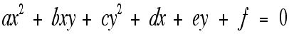
(6)
Though this equation gives the general form of a conic section or a degenerate conic section, one rarely sees conics given in this form because mathematical tools can be used to simplify the equation of the conics that one is most interested in--circles, ellipses, hyperbolas, and parabolas. However, one can see an interplay between geometry and algebra, observing that multiplying the equations of two lines together
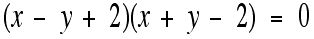
(7)
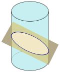
and drawing a graph of the points that satisfy this equation, will yield a "picture" of two intersecting lines. The two lines one "multiplies" to get a quadratic equation as in (7) can be identical lines or different lines, and the different lines can intersect or they can be parallel. But how can one cut the cone in Figure 4 to get two parallel lines? Notice that when the surface usually called a cylinder is cut by a plane, just like when a cone is cut by a plane, one can get "cylinder" sections that are circles or ellipses. Figure 9 shows a part of a cylinder which, when cut by a plane yields an ellipse. However, one can regard a cylinder as a "cone" where the point where the lines meet is very far away, at "infinity." One can see for this "type of cone," one can cut it to yield two parallel lines.
Figure 9 (An ellipse arises when a right circular cylinder is cut by a plane not perpendicular to the axis of the cylinder. Diagram courtesy of Wikipedia.)
One concern of analytical geometry in the 19th century was to see if one could tell what kind of conic section one was dealing with by looking at coefficients a, b, c, d, e, and f in (7). One can look at the standard form of the general quadratic equation

(8)
and determine if it has real or complex roots by looking at the quantity $b^2-4ac$. This relation is known as an "invariant." Mathematicians using "invariants" were able, based on the coefficients in (6), to determine the type of conic one was looking at, including distinguishing conics from "degenerate" conics.
Useful curves
Curves can not only be pretty but they can also be useful! The ancient Greeks and other civilizations (India, China, etc.) were curious about the paths that the planets, heavenly bodies which they realized were different from stars, moved. Ptolemy developed a "cosmology" based on the Earth being at the center of the Universe and heavenly bodies moving in circular orbits. However, by the time of Copernicus and Kepler, Ptolemy's ideas were discarded because they did not easily fit observable facts. Kepler developed "laws" for the planets which suggested that the orbits were ellipses. And there was great speculation about the curves that comets took. Furthermore, a consequence of Newton's the universal law of gravitation is that heavenly bodies such as planets in orbit around the sun, and comets travel along curves which are conic sections--parabolas, ellipses or hyperbolas. In fact, to some extent Newton the mathematician developed the Calculus to help Newton the physicist understand the laws of motion of the plants, and, therefore, provide a theoretical approach to Kepler's "empirical" laws.
Symmetry and equations
In the 19th century and earlier it was not uncommon for mathematicians to study those equations which led to attractive curves when they were represented using the Cartesian system, analytical geometry, or representing algebraic expressions visually. Geometry took an interest in symmetrical shapes very early in the history of the development of the subject, though the language we use today for symmetry did not develop until later. Today we use concepts related to geometric transformations (e.g. translations, rotations, reflections and glide reflections) and group theory (a branch of algebra) to understand or "measure" symmetry. However, the regular polyhedra and the regular tilings of the plane are early examples of calling attention to symmetrical things, where the symmetry grows out of ways of getting at the objects being studied that are not specifically rooted in knowledge of geometric transformation or group theory.
Two important types of symmetry are point symmetry and line (mirror) symmetry. Can one detect if the graph of an equation will display these types of symmetry? The answer is "yes," one can see this quite easily. The hyperbolas in Figure 8 visually show the origin as a point symmetry. The family of circles defined in (1), has both point symmetry and line symmetry.
Given an equation, if replacing x by -x and y by -y results in the same equation, the graph of the equation is symmetric in the point (0, 0).
Given an equation, if replacing x by -x results in the same equation for the graph, then the y-axis is a line of mirror symmetry.
Given an equation if replacing y by -y results in the same equation for the graph, then the x-axis is a line of mirror symmetry.
Note that the hyperbola equations in Figure 8 don't pass the test for having an axis as a line of mirror symmetry, but these hyperbolas do have the lines $y = x$ and $ y = -x$ as lines of mirror symmetry!
Functions versus equations
One of the most useful concepts that has developed in mathematics is that of a function. While functions are of interest for mathematical reasons only, they are "motivated" naturally by many applications. If one is working outside quantum physics, given a system that is being described by the variable time, the system is in only one state at a specific time--given an "input" there is exactly one output. When one inputs a particular x, say $x = u$ from the "domain" of $y = f(x)$, one gets one output from the function, denoted $f(u)$. When one has a function $y = f(x)$ and draws a graph of the pairs $(x,y)$ that satisfy this function using coordinate axes as in Figure 1, then any vertical line will intersect the graph of the function in no more than one point.
Graph picture gallery
One can look and admire the pictures at an art gallery without knowing anything about the artist, when the picture was created, or the title of the artwork. However, for pictures in an art museum the comments of the museum curators and/or the artist about his/her work can add to one's appreciation. Below is some "art" work--images of graphs of equations, mostly without comment. There is controversy about the names associated with some of these equations and sometimes the equation associated with a particular name! One way of generating curves is to look at what happens when one shape rolls or slides along another shape.
The graphs below are rendered using Wolfram/Alpha.
Folium of Descartes ("Folium" refers to something that is "leaf" shaped.)
Equation
$x^3+ y^3- 3axy = 0$
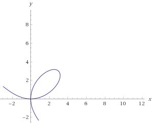
Comment: Because of the presence of the parameter a in the equation shown this is really a family of curves. Do some experiments where you vary the size and sign of the value a (e.g. $a = 6; a= -6$. What happens for $a = 0$?)
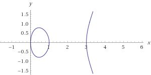
Equation:
$y^2 = x(x-1)(x-3)$
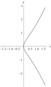
Equation:
$y^2= x(x^2+x +1)$
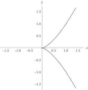
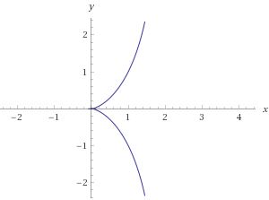
Equation:
$y^2= x^3$
Cissoid of Diocles
Equation:
$y^2= x^3/ (2-x)$
Note: This graph and the prior one have certain qualitative similarities. Can you use your knowledge of algebra to understand some ways the curves are different?
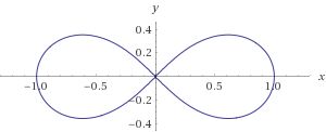
Lemniscate
Equation:
$x^2- y^2- x^4- 2x^2y^2- y^4= 0$
Equation:
$y^2= x^2(x+1)$
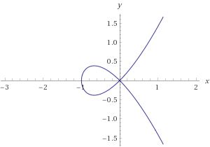
Note: This curve is qualitatively similar to the Folium shown above. Is there some "stronger" relation between these two graphs?
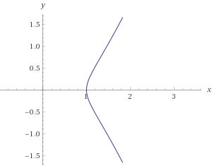
Equation:
$y^2= x^2(x-1)$
Limacon
We have looked at various pretty curves but for the most part we have drawn the graph of a single equation, though in equations (1) and (2) we looked at families of circles centered at the origin of radius r and circles centered at (5, -2) of radius r. However, sometimes when an equation has "parameters" (constant values that can be changed, thereby generating a family for different values of the parameters) the curves that we see as the parameters change are sometimes dramatically different. Such is the case with the limacon, which I will consider as a family of curves that changes as we change the value of the constant that appears in the equation of the family.
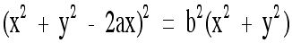
(9)
$a= 2$
$a =1/2$

Sometimes being associated with a particular intriguing equation has given a person visibility even if they are not the first to have actually studied it.
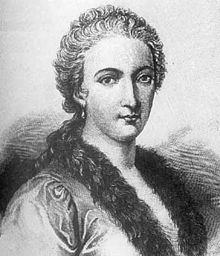
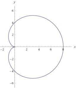
Many of the eye-catching pictures one might find appealing are associated with famous mathematicians. One such family of curves is associated with Maria Gaetana Agnesi (1718-1799). Agnesi lived, for her times, a long life. She was also a fascinating figure in the history of mathematics, being credited with having been the first person to give an integrated treatment of differential and integral calculus in one book.
Figure 10 (Portrait of Maria Gaetana Agnesi, courtesy of Wikipedia.)
Equation:
$y = 8a^3/ (x^2+ 4a^2)$
(Graph from Wolfram/Alpha)
I hope you are convinced that much is to be learned from intriguing pictures and the interplay of geometry and algebra.
Preview:
The continuation of this article about pretty pictures will discuss striking graphs in the dot/line sense meaning of the word graph. Here is a sneak preview of a graph that William Tutte (1917-2002) discovered. Although it is not the smallest such example, it was the first example of a plane 3-connected 3-valent graph that had no Hamiltonian circuit (a simple closed curve that visits each vertex of the graph once and only once). Prior to Tutte's discovery of this beautiful example, there was the chance that the 4-color conjecture (now theorem) that plane graphs can be face-colored with 4 or fewer colors might be provable by showing that all plane 3-connected 3-valent graphs HAD Hamiltonian circuits. It turned out not to be easy to prove the 4-color theorem but Kenneth Appel and Wolfgang Haken did so in 1976.
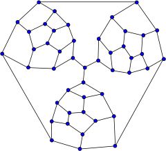
Figure 11 (Tutte graph. Courtesy of Wikipedia.)
References:
Besant, W., Roulettes and Glissetes, Deighton, Bell, London 1870.
Bix, R., Conics and Cubics, Springer, New York, 1998.
Coolidge, J., A Treatise on Algebraic Plane Curves, Dover, NY, 1959.
Hilton, H., Plane Algebraic Curves, Oxford U. Press, London, 1932.
Lawrence, J., A Catalog of Special Plane Curves, Dover, New York, 1972.
Lockwood, E., A Book of Curves, Cambridge U. Press, Cambridge, 1967.
McCarthy, J., The cissoid of Diocles, Math. Gazette 26 (1942) 12-15.
Salmon, G., Higher Plane Curves, Dublin, 1879. (Chelsea Pub. reprint, 1960.)
Walker, R., Algebraic Curves, Dover, New York, 1950.
Yates, R., A Handbook on Curves and Their Properties, 2nd ed., Edwards, Ann Arbor, 1942.
Zwikker, C., The Advanced Geometry of Plane Curves and Their Applications, Dover, New York, 1963.
Those who can access JSTOR can find some of the papers mentioned above there. For those with access, the American Mathematical Society's MathSciNet can be used to get additional bibliographic information and reviews of some of these materials. Some of the items above can be found via the ACM Portal, which also provides bibliographic services.
Joseph Malkevitch
York College (CUNY)
Email Joseph Malkevitch